Introduction to Deep Learning with PyTorch

Advanced Information Retrieval(VU) (706.705)

Markus Reiter-Haas

reiter-haas@tugraz.at

ISDS, TU Graz

2023-11-07

About Me

• University Assistant at the ISDS
  (Institute of Interactive Systems and Data Science)

• PhD candidate at Recommender Systems and Social Computing Lab at TU Graz

• Background in Web Recommender and
  Information Retrieval Systems in the industry

• Research focus: Applied Machine Learning concerning
  Computational Framing Analysis in Online Media

About today’s class

• Introduction to PyTorch library

• Fundamentals of Deep Learning

• Step-by-step build up

• Notebook provided for self-learning

• Resources (e.g., associated papers) are provided inline as link.

Learning goals

At the end of this unit, you will be able to:

• Setup a computational notebook
• Understand the basic building blocks of deep learning
• Apply PyTorch to solve machine learning problems
• List the most important tensor operations
• Know resources for future information

Recap Word2Vec

Summary last time?

• Distributional semantics

Relevance for Word2Vec

• Original Word2Vec Implementation in C
• Manual Gradient Calculation (i.e., optimization)
• Specific Code for Multithreading (i.e., parallelism)
• No separation of concerns (Architecture vs Training Procedure)

With PyTorch ~20 LoC for architecture instead of 700 incl. training
→ Input (embedding/lookup) → Projection (linear) → Output (prediction/loss)

Preliminaries

Agenda

1. Preliminaries

2. PyTorch 101

3. Learn simple functions from “scratch”

4. Typical example with NN Building Blocks

5. Discussion on Inputs and Outputs

6. Conclusion

What is Deep Learning?

“Deep learning is part of a broader family of machine learning methods, which is based on artificial neural networks with representation learning.” - Wikipedia

Simple (sigmoid) network

Illustration by Jay Alammer This work is licensed under a Creative Commons Attribution-NonCommercial-ShareAlike 4.0 International License. Alammar, J (2018). A Visual And Interactive Look at Basic Neural Network Math [Blog post]. Retrieved from https://jalammar.github.io/feedforward-neural-networks-visual-interactive/

Why deep neural networks?

• Can approximate any function.
• Reduced feature engineering.

Main Components

• LinAlg, Statistics, Optimization
• Train neural net with >= 2 layers
• Data represented as tensors

What is a Tensor?

• N-dimensional Array (0d = scalar, 1d = vector, 2d = matrix)
• In Deep Learning usually dense floating point

→ LinAlg

How to Learn from Data?

• Fitting a Function
• E.g., Linear Regression
• Minimize Error

→ Statistics

How to Find the best parameters?

• Loss Function
• Gradient Descent (SGD) + Backpropation (Chain Rule)
• Thankfully PyTorch (and similar) provide Auto Differentiation + Builtin Optimizers

→ Optimization

Types of Problems

• Prediction Variable(s): Discrete vs Continuous
• Training: Supervised vs Unsupervised

Thus 4 main types:

	Discrete	Continuous
Supervised	Classification	Regression
Unsupervised	Clustering	Dimensionality Reduction

but also special types like semi- or self-supervised.

Setup Jupyter Notebooks (local)

Install Jupyter Lab:

pip install jupyterlab
jupyter lab

Alternatives to Pip:

• Anaconda/Miniconda
• Mamba

Use Remote Services

• Colab
• Kaggle
• Many others like Paperspace

Typically not equivalent to standard Jupyter (e.g., raw cells)

Use Option to store Secrets (e.g., API tokens)

Colab

• GPU support:
  • T4 (free, supply-dependant)
  • Top Right (RAM, Disk) Dropdown - Change Runtime Type
• Google Drive can be mounted for storage
• Session must be kept active
• (Premium for better environment, e.g., GPUs)

Kaggle

• GPU support
  • P100 or T4 x2
  • Weekly Limit: 30h
  • Right Sidebar: Notebook Options –> Accelerator
• Data Persistance via Datasets
• Versioning with Run All (e.g., for long running tasks in background)
• (Extra compute via Google Cloud possible)

PyTorch 101

Agenda

1. Preliminaries

2. PyTorch 101

3. Learn simple functions from “scratch”

4. Typical example with NN Building Blocks

5. Discussion on Inputs and Outputs

6. Conclusion

Similar to Numpy

• also AutoGrad
• also GPU (CUDA) support
• also NN building blocks (later)
• Hint: numpy already is much more efficient than plain Python

Compared to Tensorflow

• Moved to foundation
• No requirement of compilation graph
• But Pytorch 2 has optional compilation: model.compile()

import torch
import matplotlib.pyplot as plt

a = torch.tensor([[1,2],[3,4]])
b = torch.tensor([[5,6],[7,8]])
c = torch.tensor([9,0])
d = torch.tensor([-1, -1, -1, -1])

a.shape, b.shape, c.shape, d.shape

(torch.Size([2, 2]), torch.Size([2, 2]), torch.Size([2]), torch.Size([4]))

Operations

• Dimensions (shape)

• Basic math

• Indexing

• Reshaping (also un/squeeze

• Broadcasting

• Combining (stack, cat)

• Statistics etc

• Properties

Basic math

a, b

(tensor([[1, 2],
         [3, 4]]),
 tensor([[5, 6],
         [7, 8]]))

Unary Operators

a.T, -a, a.log(), torch.exp(a)

(tensor([[1, 3],
         [2, 4]]),
 tensor([[-1, -2],
         [-3, -4]]),
 tensor([[0.0000, 0.6931],
         [1.0986, 1.3863]]),
 tensor([[ 2.7183,  7.3891],
         [20.0855, 54.5981]]))

Binary Operators

a+b, a-b, a*b, a/b, a@b

(tensor([[ 6,  8],
         [10, 12]]),
 tensor([[-4, -4],
         [-4, -4]]),
 tensor([[ 5, 12],
         [21, 32]]),
 tensor([[0.2000, 0.3333],
         [0.4286, 0.5000]]),
 tensor([[19, 22],
         [43, 50]]))

a@c, c@a

(tensor([ 9, 27]), tensor([ 9, 18]))

Indexing

a, b

(tensor([[1, 2],
         [3, 4]]),
 tensor([[5, 6],
         [7, 8]]))

a[0,0], a[0], a[:, 0], a[..., 0], a[0, ..., 0]

(tensor(1), tensor([1, 2]), tensor([1, 3]), tensor([1, 3]), tensor(1))

a[:,0] + b[0,:]

tensor([6, 9])

try: a[0,:,0]
except IndexError as er: print(er)

too many indices for tensor of dimension 2

Reshaping

a, d

(tensor([[1, 2],
         [3, 4]]),
 tensor([-1, -1, -1, -1]))

try: a+d
except RuntimeError as er: print(er)

The size of tensor a (2) must match the size of tensor b (4) at non-singleton dimension 1

a+d.reshape([2,2])

tensor([[0, 1],
        [2, 3]])

torch.tensor([[1, 1]]).shape, torch.tensor([1, 1]).squeeze().shape

(torch.Size([1, 2]), torch.Size([2]))

a.unsqueeze(0)

tensor([[[1, 2],
         [3, 4]]])

Broadcasting ⚠️

a+c

tensor([[10,  2],
        [12,  4]])

a+c.unsqueeze(0)

tensor([[10,  2],
        [12,  4]])

a + a.unsqueeze(0), a.unsqueeze(0) + a.unsqueeze(0)

(tensor([[[2, 4],
          [6, 8]]]),
 tensor([[[2, 4],
          [6, 8]]]))

Broadcasting rules

“It starts with the trailing (i.e. rightmost) dimension and works its way left.”

Only if:

1. they are equal, or
2. one of them is 1.

Missing Dimensions assumed to have size one.

Numpy Explanation

Combining

torch.stack([a,b]), torch.vstack([a,b]), torch.hstack([a,b]), torch.cat([a,b])

(tensor([[[1, 2],
          [3, 4]],
 
         [[5, 6],
          [7, 8]]]),
 tensor([[1, 2],
         [3, 4],
         [5, 6],
         [7, 8]]),
 tensor([[1, 2, 5, 6],
         [3, 4, 7, 8]]),
 tensor([[1, 2],
         [3, 4],
         [5, 6],
         [7, 8]]))

torch.stack([a,b]).shape, torch.vstack([a,b]).shape, torch.hstack([a,b]).shape, torch.cat([a,b]).shape

(torch.Size([2, 2, 2]),
 torch.Size([4, 2]),
 torch.Size([2, 4]),
 torch.Size([4, 2]))

Statistics

a.max(), a.max(0)

(tensor(4),
 torch.return_types.max(
 values=tensor([3, 4]),
 indices=tensor([1, 1])))

try: a.mean()
except RuntimeError as er: print(er)

mean(): could not infer output dtype. Input dtype must be either a floating point or complex dtype. Got: Long

a.float().mean()

tensor(2.5000)

Properties

Autograd + Device

• Grad_fn
• Accumulate gradients with backward

a.dtype, a.requires_grad, a.device

(torch.int64, False, device(type='cpu'))

a.to("cpu:2")

tensor([[1, 2],
        [3, 4]])

e = torch.tensor([10.0], requires_grad=True)
f = e*2
e, f

(tensor([10.], requires_grad=True), tensor([20.], grad_fn=<MulBackward0>))

print(e.grad)
f = e*2
print(e.grad)
f.backward()
print(e.grad)
f = e*2
f.backward()
print(e.grad)

None
None
tensor([2.])
tensor([4.])

with torch.no_grad():
    print(e.grad)
    f = e*2
    print(e.grad)
    print(f)
    try: f.backward()
    except RuntimeError as er: print(er, " - e:", e.grad)

tensor([4.])
tensor([4.])
tensor([20.])
element 0 of tensors does not require grad and does not have a grad_fn  - e: tensor([4.])

f = e*2
f, f.detach()

(tensor([20.], grad_fn=<MulBackward0>), tensor([20.]))

Learn simple functions from “scratch”

Agenda

1. Preliminaries

2. PyTorch 101

3. Learn simple functions from “scratch”

4. Typical example with NN Building Blocks

5. Discussion on Inputs and Outputs

6. Conclusion

def transform(x, noisy=True):
    unkown_par = 10  # to be estimated
    if noisy:
        noise = torch.randn(x.shape)
    else:
        noise = 0
    return x*unkown_par+3e-1*noise

x = torch.rand(100)
y_noisy = transform(x)
y_true = transform(x, noisy=False)

plt.scatter(x,y_noisy)
plt.plot(x,y_true, color='red')

guess = torch.tensor(5.0, requires_grad=True)
y_pred = x*guess
plt.scatter(x,y_noisy)
with torch.no_grad():
    plt.scatter(x,y_pred, color='orange')

loss = torch.abs(y_pred - y_noisy).sum()
loss.backward(retain_graph=True), loss, guess.grad

(None, tensor(250.5505, grad_fn=<SumBackward0>), tensor(-50.8152))

lr = 0.15
with torch.no_grad():
    guess -= lr * guess.grad
    guess.grad = None
guess

tensor(12.6223, requires_grad=True)

y_pred2 = x*guess
plt.scatter(x,y_noisy)
with torch.no_grad():
    plt.scatter(x,y_pred2, color='orange')

loss = torch.abs(y_pred2 - y_noisy).sum()
print(loss)
loss.backward()
print(guess.grad)
lr = 0.075
with torch.no_grad():
    guess -= lr * guess.grad
    guess.grad = None
guess

tensor(140.4753, grad_fn=<SumBackward0>)
tensor(51.0575)

tensor(8.7930, requires_grad=True)

y_pred3 = x*guess
plt.scatter(x,y_noisy)
with torch.no_grad():
    plt.scatter(x,y_pred3, color='orange')

loss = torch.abs(y_pred3 - y_noisy).sum()
loss.backward()

for i in range(1000):
    y_pred_loop = x*guess
    loss = torch.abs(y_pred_loop - y_noisy).sum()
    if i % 100 == 0:
        print(loss)
    loss.backward()
    lr *= 0.9
    with torch.no_grad():
        guess -= lr * guess.grad
        guess.grad = None
        
print(f"Final guess: {guess.item()}")
plt.scatter(x,y_noisy)
with torch.no_grad():
    plt.scatter(x,y_pred_loop, color='orange')

tensor(60.0785, grad_fn=<SumBackward0>)
tensor(19.1882, grad_fn=<SumBackward0>)
tensor(19.1882, grad_fn=<SumBackward0>)
tensor(19.1882, grad_fn=<SumBackward0>)
tensor(19.1882, grad_fn=<SumBackward0>)
tensor(19.1882, grad_fn=<SumBackward0>)
tensor(19.1882, grad_fn=<SumBackward0>)
tensor(19.1882, grad_fn=<SumBackward0>)
tensor(19.1882, grad_fn=<SumBackward0>)
tensor(19.1882, grad_fn=<SumBackward0>)
Final guess: 9.930237770080566

Observations

• We need a smooth loss function (not right/wrong)
• Importance of learning rate (hint scheduling)
• Convergence behavior
• Overfitting?

Typical example with NN Building Blocks

Agenda

1. Preliminaries

2. PyTorch 101

3. Learn simple functions from “scratch”

4. Typical example with NN Building Blocks

5. Discussion on Inputs and Outputs

6. Conclusion

torch.manual_seed(42)  # For reproducibility

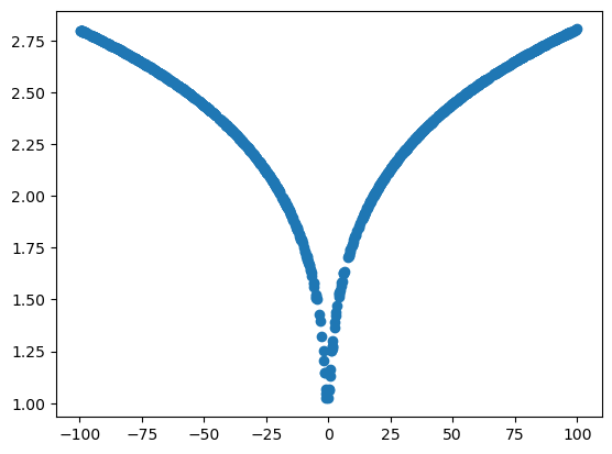
def unknown_function(x):  # We want to approximate it, but assume that we don't know it.
    return (3*x**2+2*x+1)**0.1

random_numbers = torch.rand(1000)
input_numbers = random_numbers * 200 - 100  # rescaled between -100 and 100
target_numbers = unknown_function(input_numbers)

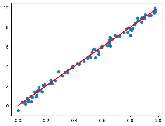
plt.scatter(x=input_numbers, y=target_numbers)

<matplotlib.collections.PathCollection at 0x7e9880a01660>

Unknown function to be learned.

Common building blocks

• Layers of linear units with pointwise non-linearity
• ReLU Activations
• Batches

from torch import nn

class SimpleModel(nn.Module):
    def __init__(self):
        super().__init__()
        self.linear_relu_stack = nn.Sequential(
            nn.Linear(1, 50),  # Usually we have more inputs, i.e., a more complex problem to solve.
            nn.ReLU(),  # Important between linear layers
            nn.Linear(50, 50),  # Multiple stacked layers
            nn.ReLU(),  
            nn.Linear(50, 1)  # Dimensions must match
        )

    def forward(self, x):
        logits = self.linear_relu_stack(x)
        return logits

example_model = SimpleModel()

def plot_predictions(inp, model):
    with torch.no_grad():  # No gradients will be calculated
        inp_reshaped = inp.unsqueeze(-1)  # Note that we make sure that the dimensions match (at least broadcastable)
        preds = example_model(inp_reshaped)

        plt.scatter(inp, preds)  
    
#  Output random by default
plot_predictions(input_numbers, example_model)

# Hyperparameters
epochs = 30
loss_fn = nn.MSELoss()  # Depends on the problem
optimizer = torch.optim.SGD(example_model.parameters(), lr=1e-7)  # Especially in simple optimizers, learning rate is crucial

# Training loop (without evaluation)
for epoch in range(epochs):
    total_loss = 0
    batch_size = 10
    num_chunks = int(len(input_numbers)/batch_size)
    
    for batch_input, batch_target in zip(  # We use batches to speed up peformance, but do not load the whole dataset at once.
        torch.chunk(input_numbers, num_chunks), 
        torch.chunk(target_numbers, num_chunks)
    ):  
        # Compute prediction error
        preds = example_model(batch_input.unsqueeze(-1)).squeeze()
        loss = loss_fn(preds, batch_target)
        
        # Backpropagation
        optimizer.zero_grad()
        loss.backward()
        optimizer.step()
        
        total_loss += loss.item()
    
    print(total_loss/num_chunks, end=" --> ")

# For demonstration
plot_predictions(input_numbers, example_model)

28.07128987312317 --> 23.263446702957154 --> 19.3093986082077 --> 16.053855652809144 --> 13.371083998680115 --> 11.158774189949035 --> 9.333402314186095 --> 7.826536514759064 --> 6.582430763244629 --> 5.555449168682099 --> 4.707653863430023 --> 4.0077322745323185 --> 3.429861843585968 --> 2.9527618789672854 --> 2.5588334500789642 --> 2.233610113859177 --> 1.9650949335098267 --> 1.7433959233760834 --> 1.560362531542778 --> 1.4092276573181153 --> 1.2843796110153198 --> 1.1812364035844802 --> 1.0960449695587158 --> 1.0256566640734672 --> 0.9674729079008102 --> 0.9193610382080079 --> 0.8795562756061553 --> 0.8466201943159103 --> 0.8193569293618203 --> 0.7967806303501129 --> 

Loss Function

\[ MSE = \frac{1}{n} \sum^n_{i=1} (y_i - \hat{y}_i)^2 \]

Discussion on Inputs and Outputs

Agenda

1. Preliminaries

2. PyTorch 101

3. Learn simple functions from “scratch”

4. Typical example with NN Building Blocks

5. Discussion on Inputs and Outputs

6. Conclusion

DataSet Splits

• Train Set
• Valid/Dev Set
• Test Set

For instance, 80/10/10 random split.

❗️Major Pitfall in Practice

Relating back to Word2Vec

• Words for NN? One-hot [0, 0, 1, 0,] or Embeddings [0.3, 0.1, -0.7, 0.6]. Can be jointly learned.
• Categorical loss such as CrossEntropyLoss, often with Softmax (see Word2Vec).

\[ BCE = \frac{1}{n} \sum^n_{i=1} y_i \cdot \log\hat{y}_i + (1 - y_i) \cdot \log(1 - \hat{y}_i) \]

# https://towardsdatascience.com/word2vec-with-pytorch-implementing-original-paper-2cd7040120b0
import torch.nn as nn 
EMBED_DIMENSION = 300 
EMBED_MAX_NORM = 1 
class CBOW_Model(nn.Module):
    def __init__(self, vocab_size: int):
        super(CBOW_Model, self).__init__()
        self.embeddings = nn.Embedding(
            num_embeddings=vocab_size,
            embedding_dim=EMBED_DIMENSION,
            max_norm=EMBED_MAX_NORM,
        )
        self.linear = nn.Linear(
            in_features=EMBED_DIMENSION,
            out_features=vocab_size,
        )
     def forward(self, inputs_):
        x = self.embeddings(inputs_)
        x = x.mean(axis=1)
        x = self.linear(x)
        return x

Conclusion

Agenda

1. Preliminaries

2. PyTorch 101

3. Learn simple functions from “scratch”

4. Typical example with NN Building Blocks

5. Discussion on Inputs and Outputs

6. Conclusion

Summary

• From Tensor Operations to Model Training
• Common building blocks, such as Layers
• Importance of Input, Output, and Hyperparameters

Recommended Activities

• Try running and adapting on your own
• Jalammer Blog for major concepts
• PyTorch Quickstart
• Create your own (first) deep learning model

Key Take-Aways

• Simplify problems
• Guided by data
• Implicit operations (gradients) performed by libraries

Questions?

Next Time: Sequence Modeling

cnn = nn.Conv1d(16, 33, 3, stride=2)
rnn = nn.RNN(10, 20, 2)
lstm = nn.LSTM(10, 20, 2)
gru = nn.GRU(10, 20, 2)