Transformers 4 IR

Advanced Information Retrieval(VU) (706.705)

Markus Reiter-Haas

ISDS, TU Graz

2023-11-28, 2023-12-05

About today’s class

  • Learn about Transformers and its uses for IR
  • Hands-on step-by-step tutorial on how to performan an IR experiment
  • Should provide guidance for practicals
  • We will focus on BERT (likely the most popular), but knowledges translates to other Transformers as well
  • Based on BERT 4 Text Ranking
  • Showcase sBERT and BERTopic libraries (build upon HuggingFace and PyTorch)
  • Illustrations will link to Jay Alammer Blog and sBERT Docs
  • Resources (e.g., associated papers) are provided inline as link.

Learning goals

At the end of this unit, you will be able to:

  • setup and perform an IR experiment including preprocessing and analysis
  • apply transformers to solve IR problems, such as text (re-)ranking
  • understand how transformers can be used to improve text retrieval
  • list well-known architectures and their use cases
  • develop suitable training procedures for IR tasks
  • know best practices and pitfalls in IR evaluation

Recap Neural Retrieval

  • Neural networks applied to IR tasks.
  • For instance, estimate relevance.
  • Often heavily relies on embeddings.

Neural Network Components

  • Architecture
  • Model (+ weights)
  • Loss
  • Optimizer
  • Optional Scheduler

Transformer by Examples

Agenda

  1. Transformers 4 IR

  2. Transformer by Examples

  3. Conducting an IR experiment

  4. Analysis - BERTopic Showcase

  5. BERT 4 Reranking - monoBERT (= Cross-encoder)

  6. What is a Transformer? (High-level Overview)

  7. BERT 4 Retrieval - Representation-based (= Bi-encoder)

  8. Discussion

Pretrained Transformer

%pip install -Uq sentence-transformers faiss-cpu accelerate hdbscan bertopic evaluate kaleido datasets>=2.11
from transformers import AutoTokenizer, AutoModel, AutoModelForSequenceClassification
from transformers import pipeline
import numpy as np
import torch

examples = ["I love you.", "I hate you.", "I see you."]
trans_tokenizer = AutoTokenizer.from_pretrained("cardiffnlp/twitter-roberta-base-sentiment")
trans_model = AutoModelForSequenceClassification.from_pretrained("cardiffnlp/twitter-roberta-base-sentiment")
trans_model(**trans_tokenizer(examples, return_tensors="pt"))
SequenceClassifierOutput(loss=None, logits=tensor([[-2.0218, -0.3980,  3.0771],
        [ 2.8151, -0.5906, -2.0748],
        [-0.1817,  0.9144, -0.3362]], grad_fn=<AddmmBackward0>), hidden_states=None, attentions=None)
# Alternatively load fixed pipeline
pipeline("text-classification", model="cardiffnlp/twitter-roberta-base-sentiment")(examples)
[{'label': 'LABEL_2', 'score': 0.9642633199691772},
 {'label': 'LABEL_0', 'score': 0.9608864784240723},
 {'label': 'LABEL_1', 'score': 0.6171057820320129}]
trans_tokenizer(examples)
{'input_ids': [[0, 100, 657, 47, 4, 2], [0, 100, 4157, 47, 4, 2], [0, 100, 192, 47, 4, 2]], 'attention_mask': [[1, 1, 1, 1, 1, 1], [1, 1, 1, 1, 1, 1], [1, 1, 1, 1, 1, 1]]}

Consider the embeddings only

trans_model_wo_head = trans_model.roberta  # No trans_model.classifier
res = trans_model_wo_head(**trans_tokenizer(examples, return_tensors="pt")).last_hidden_state
np.array(trans_tokenizer(examples)["input_ids"])[:, 3]
array([47, 47, 47])
res[:, 3, :8]  # Completely different
tensor([[ 0.2013,  1.1354, -0.4476, -0.4864,  1.4788,  0.8109,  0.3484, -0.5514],
        [-0.2421,  0.2407,  0.1613, -0.7413,  1.2675, -1.1970,  0.9893, -0.3319],
        [-0.4125, -0.4480,  0.3700, -0.6575,  0.8338, -0.1514,  0.4230, -0.3423]],
       grad_fn=<SliceBackward0>)
res[0].mean(0).shape  # simple pooling of first example
torch.Size([768])
id_map = {
    0: "love",
    1: "hate",
    2: "see ",
}
def pairwise_cosine_sim(res):
    import torch
    from torch import nn
    cos_sim = torch.nn.CosineSimilarity(dim=0)
    for i in range(3):
        for j in range(3):
            if i == j:  # always 1
                continue
            if i > j:  # symmetric relation
                continue
            c = cos_sim(res[i].mean(0), res[j].mean(0))
            print(id_map[i], id_map[j], c)
            
pairwise_cosine_sim(res)  # While all show similarity, we observe some expected differences
love hate tensor(0.2491, grad_fn=<SumBackward1>)
love see  tensor(0.5104, grad_fn=<SumBackward1>)
hate see  tensor(0.6279, grad_fn=<SumBackward1>)

Comparison to Word2Vec

# Load tokenizer and model but take only Word2Vec layer
REPO_NAME = "vocab-transformers/distilbert-word2vec_256k-MLM_250k"

w2v_tokenizer = AutoTokenizer.from_pretrained(REPO_NAME)
w2v_model = AutoModel.from_pretrained(REPO_NAME)._modules["embeddings"].word_embeddings
t = torch.tensor(w2v_tokenizer(examples).input_ids)
t, w2v_tokenizer.convert_ids_to_tokens(t[:, 3])
(tensor([[    1,    75, 26564, 25776,    42,     2],
         [    1,    75, 33141, 25776,    42,     2],
         [    1,    75, 26213, 25776,    42,     2]]),
 ['you', 'you', 'you'])
res2 = w2v_model(t)
res2[:, 3, :8]  # all the same
tensor([[-0.0596, -0.0382, -0.0150, -0.0114, -0.0367, -0.0157, -0.0453,  0.0235],
        [-0.0596, -0.0382, -0.0150, -0.0114, -0.0367, -0.0157, -0.0453,  0.0235],
        [-0.0596, -0.0382, -0.0150, -0.0114, -0.0367, -0.0157, -0.0453,  0.0235]],
       grad_fn=<SliceBackward0>)
pairwise_cosine_sim(res2)  # All sentences are seen as almost identical.
love hate tensor(0.9487, grad_fn=<SumBackward1>)
love see  tensor(0.9415, grad_fn=<SumBackward1>)
hate see  tensor(0.9334, grad_fn=<SumBackward1>)

Application Examples of Transformers

So far we have seen text classification and embeddings (i.e., base encoders without head, for instance as textual similarity).

Text Generation (GPT)

The well known example: ChatGPT got lots of attention from a broader audience.
Also due to, statements about “sentient AI”.

pipeline("text-generation", model="gpt2")(
    "My name is Mariama, my favorite"
)
[{'generated_text': 'My name is Mariama, my favorite anime about me."\n\nHer husband was a classmate of Natsuki\'s, and the two were "fascinating and adorable friends." He told Natsuki that he had never met his own husband before:'}]

Mask Filling

This is often used for pretrainig of models, e.g., in BERT.

pipeline("fill-mask", "bert-base-uncased")(
    "Paris is the [MASK] of France."
)
[{'score': 0.9969370365142822,
  'token': 3007,
  'token_str': 'capital',
  'sequence': 'paris is the capital of france.'},
 {'score': 0.0005914860521443188,
  'token': 2540,
  'token_str': 'heart',
  'sequence': 'paris is the heart of france.'},
 {'score': 0.0004378748417366296,
  'token': 2415,
  'token_str': 'center',
  'sequence': 'paris is the center of france.'},
 {'score': 0.0003378352848812938,
  'token': 2803,
  'token_str': 'centre',
  'sequence': 'paris is the centre of france.'},
 {'score': 0.0002699583419598639,
  'token': 2103,
  'token_str': 'city',
  'sequence': 'paris is the city of france.'}]

Token Classification

pipeline("token-classification", model="dslim/bert-base-NER")(
    "My name is Sarah and I live in London"
)
[{'entity': 'B-PER',
  'score': 0.99854773,
  'index': 4,
  'word': 'Sarah',
  'start': 11,
  'end': 16},
 {'entity': 'B-LOC',
  'score': 0.9996215,
  'index': 9,
  'word': 'London',
  'start': 31,
  'end': 37}]

Zero Shot Classification

classifier = pipeline("zero-shot-classification",
                      model="facebook/bart-large-mnli")
sequence_to_classify = "one day I will see the world"
candidate_labels = ['travel', 'cooking', 'dancing']
classifier(sequence_to_classify, candidate_labels)
{'sequence': 'one day I will see the world',
 'labels': ['travel', 'dancing', 'cooking'],
 'scores': [0.9938650727272034, 0.003273805370554328, 0.0028610355220735073]}
candidate_labels = ['travel', 'cooking', 'dancing', 'exploration']
classifier(sequence_to_classify, candidate_labels)
{'sequence': 'one day I will see the world',
 'labels': ['travel', 'exploration', 'dancing', 'cooking'],
 'scores': [0.7957563400268555,
  0.199331596493721,
  0.0026212322991341352,
  0.0022907406091690063]}
candidate_labels = ['travel', 'cooking', 'dancing', 'exploration']
classifier(sequence_to_classify, candidate_labels, multi_label=True)
{'sequence': 'one day I will see the world',
 'labels': ['travel', 'exploration', 'dancing', 'cooking'],
 'scores': [0.994511067867279,
  0.9383884072303772,
  0.005706198047846556,
  0.0018192853312939405]}

Question Answering (extractive)

pipeline("question-answering", model="deepset/minilm-uncased-squad2")(
    question="Where do I live?",
    context="My name is Sarah and I live in London"
)
{'score': 0.9948917031288147, 'start': 31, 'end': 37, 'answer': 'London'}

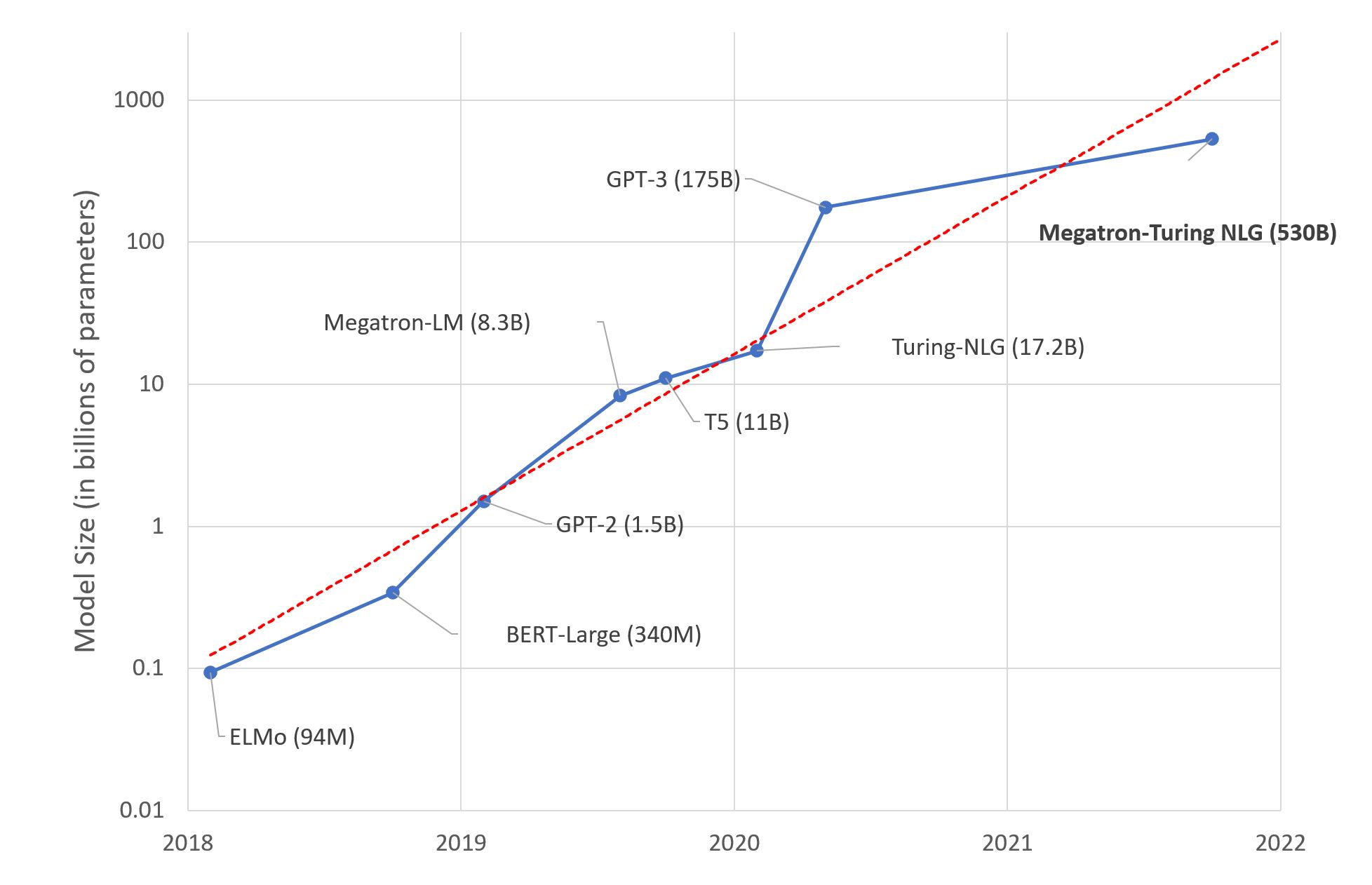
History of Transformers

Word2Vec 2013 → Attention 2014 → Transformers 2017


Gradual Improvements:

  • BERT (2018), BART (2019), GPT (1-3, 2018-2020)
  • Vision Transformers (2020)
  • Failed Attempts at LLMs (Galactica 2022, 3 days)

Until:

  • ChatGPT released on November 30, 2022
  • Many from Industry since (Bard, Llama)
  • Towards Open-Source (Alpaca, Llama2, Falcon)

Fig.: Models Size over Time

Conducting an IR experiment

Agenda

  1. Transformers 4 IR

  2. Transformer by Examples

  3. Conducting an IR experiment

  4. Analysis - BERTopic Showcase

  5. BERT 4 Reranking - monoBERT (= Cross-encoder)

  6. What is a Transformer? (High-level Overview)

  7. BERT 4 Retrieval - Representation-based (= Bi-encoder)

  8. Discussion

Typical pipeline:

  • Loading and processing a dataset
  • Implement algorithms and baselines.
  • Running algorithms (simulating real-world application).
  • Evaluating the results (beyond loss).
  • Analysing the results.
  • Optional: optimize and put into production.

Setup (IR dataset)

This notebook was developed on Kaggle. As Kaggle provides a basic stable environment, no tinkering is required (i.e., setup Jupyter, Conda/Pip, Python Environment).

Let’s first setup the required libraries (usually iteratively updated).

from datasets import load_dataset, DatasetDict
import sentence_transformers
import sentence_transformers.cross_encoder.evaluation
from sentence_transformers import SentenceTransformer, CrossEncoder, InputExample  # High-level sentence encoders.
import sentence_transformers.models as models
import sentence_transformers.losses as losses
import torch
from torch.utils.data import Dataset, DataLoader
from tqdm import tqdm  # Enables progress bars
import pandas as pd
import matplotlib.pyplot as plt

import os
os.environ["TOKENIZERS_PARALLELISM"] = "false"

QUICK_RUN = False  # Config setting to switch between foreground (subset) and background (full-dataset) running

Choosing (finding) the dataset.

We will perform document retrieval and ranking. Hence, we choose a benchmark dataset in this domain on Scientific documents.

# https://aclanthology.org/2020.acl-main.207/
# https://arxiv.org/abs/2104.08663
queries = load_dataset("BeIR/scidocs", "queries", split="queries")
docs = load_dataset("BeIR/scidocs", "corpus", split="corpus")
qrels = load_dataset("BeIR/scidocs-qrels", delimiter="\t", split="test")
len(queries), len(docs), len(qrels), len(set(qrels["query-id"])), len(set(qrels["corpus-id"]))
(1000, 25657, 29928, 1000, 25657)

Structure

In IR, we have a query, a collection of documents and a assignment of relevancy between (some) queries and documents. This can be seen by the way the dataset is structured.

queries, docs, qrels
(Dataset({
     features: ['_id', 'title', 'text'],
     num_rows: 1000
 }),
 Dataset({
     features: ['_id', 'title', 'text'],
     num_rows: 25657
 }),
 Dataset({
     features: ['query-id', 'corpus-id', 'score'],
     num_rows: 29928
 }))

Preprocessing. Sparsity. Cold-start problem. Keep in mind the tasks.

Our dataset already has a natural representation. We could still perform filtering. We must ensure that no information is lost.

# For demonstration purposes only
if QUICK_RUN:
    queries = queries.select(range(100))
    docs = docs.select(range(2500))
    qrels = qrels.filter(lambda x: x["query-id"] in queries["_id"] and x["corpus-id"] in docs["_id"])

Train, validation, test set.

This step is very important.

  • Train for algorithm parameter estimation.
  • Valid-ation (also called dev-elopment) for finding a good model (e.g., hyperparameter optimization, cross-validation).
  • Test (also called eval-uation) only used for evaluation at the very end.

Sometimes datasets have predefined splits that can be used.

# 90% train, 10% test + validation
train_testvalid = qrels.train_test_split(test_size=0.1, seed=1)
# Split the 10% test + valid in half test, half valid
test_valid = train_testvalid['test'].train_test_split(test_size=0.5, seed=1)
# gather everyone if you want to have a single DatasetDict
train_test_valid_dataset = DatasetDict({
    'train': train_testvalid['train'],
    'test': test_valid['test'],
    'valid': test_valid['train']})
train_test_valid_dataset
DatasetDict({
    train: Dataset({
        features: ['query-id', 'corpus-id', 'score'],
        num_rows: 26935
    })
    test: Dataset({
        features: ['query-id', 'corpus-id', 'score'],
        num_rows: 1497
    })
    valid: Dataset({
        features: ['query-id', 'corpus-id', 'score'],
        num_rows: 1496
    })
})

Splitting methods

  • depend on the task
  • random sometimes not feasible -> data leakage

Common alternative splitting options:

  • time-based
  • session-based
  • user-based

Analysis - BERTopic Showcase

Agenda

  1. Transformers 4 IR

  2. Transformer by Examples

  3. Conducting an IR experiment

  4. Analysis - BERTopic Showcase

  5. BERT 4 Reranking - monoBERT (= Cross-encoder)

  6. What is a Transformer? (High-level Overview)

  7. BERT 4 Retrieval - Representation-based (= Bi-encoder)

  8. Discussion

First, we will analyze the data.
For the start let’s just look at some example relevance assignments and their associated content.

def get_triple_for_example(example):
    q = queries[queries["_id"].index(example["query-id"])]["text"]
    d = docs[docs["_id"].index(example["corpus-id"])]["title"]
    r = example["score"]
    return q, d, r

ex0 = get_triple_for_example(train_test_valid_dataset["test"][0])
ex1 = get_triple_for_example(train_test_valid_dataset["test"][1])
ex0, ex1
(('Provable data possession at untrusted stores',
  'StreamOp: An Innovative Middleware for Supporting Data Management and Query Functionalities over Sensor Network Streams Efficiently',
  0),
 ('Rumor Detection and Classification for Twitter Data',
  'Thumbs Up or Thumbs Down? Semantic Orientation Applied to Unsupervised Classification of Reviews',
  1))

Label Distribution

An important aspect to consider.
What would be an implication of an imbalanced dataset?

import evaluate
# Here we use evaluate library
# Alternatively, implement on your own with scipy.stats and collections.Counter
label_dist = evaluate.load("evaluate-measurement/label_distribution")
label_dist.compute(data=train_test_valid_dataset["train"]["score"]), label_dist.compute(data=train_test_valid_dataset["valid"]["score"]), label_dist.compute(data=train_test_valid_dataset["test"]["score"])
({'label_distribution': {'labels': [1, 0],
   'fractions': [0.16461852608130684, 0.8353814739186931]},
  'label_skew': 1.8087864265977875},
 {'label_distribution': {'labels': [0, 1],
   'fractions': [0.8348930481283422, 0.16510695187165775]},
  'label_skew': 1.8040061996868444},
 {'label_distribution': {'labels': [0, 1],
   'fractions': [0.8350033400133601, 0.16499665998663995]},
  'label_skew': 1.8050841379113802})

Content

Next, we will look at the content via topic modeling.
We use a recent model called BERTopic (2022).

docs.map(lambda x: {"title_text": x["title"] + ": " + x["text"]})["title_text"][:2]
['A hybrid of genetic algorithm and particle swarm optimization for recurrent network design: An evolutionary recurrent network which automates the design of recurrent neural/fuzzy networks using a new evolutionary learning algorithm is proposed in this paper. This new evolutionary learning algorithm is based on a hybrid of genetic algorithm (GA) and particle swarm optimization (PSO), and is thus called HGAPSO. In HGAPSO, individuals in a new generation are created, not only by crossover and mutation operation as in GA, but also by PSO. The concept of elite strategy is adopted in HGAPSO, where the upper-half of the best-performing individuals in a population are regarded as elites. However, instead of being reproduced directly to the next generation, these elites are first enhanced. The group constituted by the elites is regarded as a swarm, and each elite corresponds to a particle within it. In this regard, the elites are enhanced by PSO, an operation which mimics the maturing phenomenon in nature. These enhanced elites constitute half of the population in the new generation, whereas the other half is generated by performing crossover and mutation operation on these enhanced elites. HGAPSO is applied to recurrent neural/fuzzy network design as follows. For recurrent neural network, a fully connected recurrent neural network is designed and applied to a temporal sequence production problem. For recurrent fuzzy network design, a Takagi-Sugeno-Kang-type recurrent fuzzy network is designed and applied to dynamic plant control. The performance of HGAPSO is compared to both GA and PSO in these recurrent networks design problems, demonstrating its superiority.',
 'A Hybrid EP and SQP for Dynamic Economic Dispatch with Nonsmooth Fuel Cost Function: Dynamic economic dispatch (DED) is one of the main functions of power generation operation and control. It determines the optimal settings of generator units with predicted load demand over a certain period of time. The objective is to operate an electric power system most economically while the system is operating within its security limits. This paper proposes a new hybrid methodology for solving DED. The proposed method is developed in such a way that a simple evolutionary programming (EP) is applied as a based level search, which can give a good direction to the optimal global region, and a local search sequential quadratic programming (SQP) is used as a fine tuning to determine the optimal solution at the final. Ten units test system with nonsmooth fuel cost function is used to illustrate the effectiveness of the proposed method compared with those obtained from EP and SQP alone.']
model_name = 'sentence-transformers/all-MiniLM-L6-v2'
from bertopic import BERTopic
from bertopic.vectorizers import ClassTfidfTransformer
import plotly

docs_for_analysis = docs.map(lambda x: {"title_text": x["title"] + ": " + x["text"]})["title_text"]
topic_model = BERTopic(embedding_model=model_name, ctfidf_model=ClassTfidfTransformer(reduce_frequent_words=True))
topic_model.fit(docs_for_analysis)
topic_model.get_topic_info().head()
Topic Count Name Representation Representative_Docs
0 -1 8734 -1_personality_object_health_objects [personality, object, health, objects, query, ... [The Cascade-Correlation Learning Architecture...
1 0 327 0_antenna_patch_radiation_polarized [antenna, patch, radiation, polarized, microst... [Low-Cost High-Gain and Broadband Substrate- I...
2 1 326 1_reinforcement_rl_policy_reward [reinforcement, rl, policy, reward, agent, cri... [GQ ( λ ) : A general gradient algorithm for t...
3 2 306 2_cortex_cortical_brain_fmri [cortex, cortical, brain, fmri, hippocampus, f... [Cortical hubs revealed by intrinsic functiona...
4 3 241 3_imagenet_accelerator_dropout_dnns [imagenet, accelerator, dropout, dnns, cifar, ... [Incremental Network Quantization: Towards Los...

Explain Embeddings (UMAP plot)

topic_model.reduce_topics(docs_for_analysis, nr_topics=15)
fig = topic_model.visualize_documents(docs_for_analysis)
# plotly.offline.plot(fig, filename='bertopic_doc_embeddings.svg', image="svg")
fig.write_image("bertopic_doc_embeddings.svg")
from IPython.display import SVG
SVG('bertopic_doc_embeddings.svg')

BERT 4 Reranking - monoBERT (= Cross-encoder)

Agenda

  1. Transformers 4 IR

  2. Transformer by Examples

  3. Conducting an IR experiment

  4. Analysis - BERTopic Showcase

  5. BERT 4 Reranking - monoBERT (= Cross-encoder)

  6. What is a Transformer? (High-level Overview)

  7. BERT 4 Retrieval - Representation-based (= Bi-encoder)

  8. Discussion

Overview

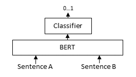
Idea:

  • Concat and predict.
  • Can directly use pretrained architectures.
  • Just fine-tuning required.

Cross Encoder
from collections import defaultdict

class IRDataset(Dataset):
    def __init__(self, queries_ds, docs_ds, qrel_ds, mode="cross"):
        self.mode = mode
        
        qrels = defaultdict(set)
        
        def transform(x):
            q, d, r = x["query-id"], x["corpus-id"], x["score"]
            
            q_idx = queries_ds["_id"].index(q)
            x["query_text"] = queries_ds[q_idx]["text"]
            d_idx = docs_ds["_id"].index(d)
            x["doc_content"] = docs_ds[d_idx]["title"] + ": " + docs_ds[d_idx]["text"]
            x["label"] = float(r)
            
            if r:
                qrels[q].add(d)
            
            return x
        
        qrel_ds = qrel_ds.map(transform)
            
        self.q_ids = qrel_ds["query-id"]
        self.d_ids = qrel_ds["corpus-id"]
        self.qrels = qrels
                
        self.queries = qrel_ds["query_text"]
        self.docs = qrel_ds["doc_content"]
        self.labels = qrel_ds["label"]

    def __getitem__(self, idx):
        qs = self.queries[idx]
        ds = self.docs[idx]
        if self.mode == "rep":
            if type(idx) is int:
                text_list = [{"query": qs}, {"doc": ds}]
            else:
                text_list = [[{"query": q} for q in qs], [{"doc": d} for d in ds]]
            return InputExample(texts=text_list, label=self.labels[idx])
        return InputExample(texts=[qs, ds], label=self.labels[idx])
    
    def set_mode(self, mode):
        self.mode = mode

    def __len__(self):
        return len(self.labels)
train_ds = IRDataset(queries, docs, train_test_valid_dataset["train"])
valid_ds = IRDataset(queries, docs, train_test_valid_dataset["valid"])
train_ds[0].__dict__
{'guid': '',
 'texts': ['Toward an IT governance maturity self-assessment model using EFQM and CobiT',
  'A maturity model for information governance: Information Governance (IG) as defined by Gartner is the “specification of decision rights and an accountability framework to encourage desirable behavior in the valuation, creation, storage, use, archival and deletion of information. Includes the processes, roles, standards and metrics that ensure the effective and efficient use of information in enabling an organization to achieve its goals”. In this paper, we present how to create an IG maturity model based on existing reference documents. The process is based on existing maturity model development methods. These methods allow for a systematic approach to maturity model development backed up by a well-known and proved scientific research method called Design Science Research. Then, based on the maturity model proposed in this paper, an assessment is conducted and the results are presented, this assessment was conducted as a self-assessment in the context of the EC-funded E-ARK project for the seven pilots of the project. The main conclusion from this initial assessment is that there is much room for improvement with most pilots achieving results between maturity level two and three. As future work, the goal is to analyze other references from different domains, such as, records management. These references will enhance, detail and help develop the maturity model making it even more valuable for all types of organization that deal with information governance.'],
 'label': 1.0}
monoBERT = CrossEncoder(model_name, # We use cross-encoder as monoBERT example
                     num_labels=1, # Perform binary classification
                     device=None,  # Will use CUDA if available
                    )
monoBERT.predict([ex0[:2], ex1[:2]])
array([0.5064283, 0.5081911], dtype=float32)
print(train_ds[0])
<InputExample> label: 1.0, texts: Toward an IT governance maturity self-assessment model using EFQM and CobiT; A maturity model for information governance: Information Governance (IG) as defined by Gartner is the “specification of decision rights and an accountability framework to encourage desirable behavior in the valuation, creation, storage, use, archival and deletion of information. Includes the processes, roles, standards and metrics that ensure the effective and efficient use of information in enabling an organization to achieve its goals”. In this paper, we present how to create an IG maturity model based on existing reference documents. The process is based on existing maturity model development methods. These methods allow for a systematic approach to maturity model development backed up by a well-known and proved scientific research method called Design Science Research. Then, based on the maturity model proposed in this paper, an assessment is conducted and the results are presented, this assessment was conducted as a self-assessment in the context of the EC-funded E-ARK project for the seven pilots of the project. The main conclusion from this initial assessment is that there is much room for improvement with most pilots achieving results between maturity level two and three. As future work, the goal is to analyze other references from different domains, such as, records management. These references will enhance, detail and help develop the maturity model making it even more valuable for all types of organization that deal with information governance.
train_dl = DataLoader(train_ds, batch_size=32)
# We need sentence pairs format for the library here.
# valid_dl = DataLoader(valid_ds, batch_size=32)
sentence_pairs = list(zip(valid_ds.queries, valid_ds.docs))
labels = valid_ds.labels
len(train_dl)
842
monoBERT.model
BertForSequenceClassification(
  (bert): BertModel(
    (embeddings): BertEmbeddings(
      (word_embeddings): Embedding(30522, 384, padding_idx=0)
      (position_embeddings): Embedding(512, 384)
      (token_type_embeddings): Embedding(2, 384)
      (LayerNorm): LayerNorm((384,), eps=1e-12, elementwise_affine=True)
      (dropout): Dropout(p=0.1, inplace=False)
    )
    (encoder): BertEncoder(
      (layer): ModuleList(
        (0-5): 6 x BertLayer(
          (attention): BertAttention(
            (self): BertSelfAttention(
              (query): Linear(in_features=384, out_features=384, bias=True)
              (key): Linear(in_features=384, out_features=384, bias=True)
              (value): Linear(in_features=384, out_features=384, bias=True)
              (dropout): Dropout(p=0.1, inplace=False)
            )
            (output): BertSelfOutput(
              (dense): Linear(in_features=384, out_features=384, bias=True)
              (LayerNorm): LayerNorm((384,), eps=1e-12, elementwise_affine=True)
              (dropout): Dropout(p=0.1, inplace=False)
            )
          )
          (intermediate): BertIntermediate(
            (dense): Linear(in_features=384, out_features=1536, bias=True)
            (intermediate_act_fn): GELUActivation()
          )
          (output): BertOutput(
            (dense): Linear(in_features=1536, out_features=384, bias=True)
            (LayerNorm): LayerNorm((384,), eps=1e-12, elementwise_affine=True)
            (dropout): Dropout(p=0.1, inplace=False)
          )
        )
      )
    )
    (pooler): BertPooler(
      (dense): Linear(in_features=384, out_features=384, bias=True)
      (activation): Tanh()
    )
  )
  (dropout): Dropout(p=0.1, inplace=False)
  (classifier): Linear(in_features=384, out_features=1, bias=True)
)
monoBERT.__dict__.keys()
dict_keys(['config', 'model', 'tokenizer', 'max_length', '_target_device', 'default_activation_function'])
class_evaluator = sentence_transformers.cross_encoder.evaluation.CEBinaryClassificationEvaluator(sentence_pairs, labels, show_progress_bar=True)
monoBERT.fit(train_dataloader=train_dl,
          loss_fct=None,  # uses nn.BCEWithLogitsLoss() 
          evaluator=class_evaluator,
          epochs=5, 
          optimizer_class=torch.optim.AdamW,
          show_progress_bar=True,
          save_best_model=True,
          output_path="./",
        )
# Tip: look at CUDA GPU.
!nvidia-smi
Mon Nov 20 16:22:17 2023       
+-----------------------------------------------------------------------------+
| NVIDIA-SMI 470.161.03   Driver Version: 470.161.03   CUDA Version: 11.4     |
|-------------------------------+----------------------+----------------------+
| GPU  Name        Persistence-M| Bus-Id        Disp.A | Volatile Uncorr. ECC |
| Fan  Temp  Perf  Pwr:Usage/Cap|         Memory-Usage | GPU-Util  Compute M. |
|                               |                      |               MIG M. |
|===============================+======================+======================|
|   0  Tesla P100-PCIE...  Off  | 00000000:00:04.0 Off |                    0 |
| N/A   70C    P0    54W / 250W |   9533MiB / 16280MiB |      0%      Default |
|                               |                      |                  N/A |
+-------------------------------+----------------------+----------------------+
                                                                               
+-----------------------------------------------------------------------------+
| Processes:                                                                  |
|  GPU   GI   CI        PID   Type   Process name                  GPU Memory |
|        ID   ID                                                   Usage      |
|=============================================================================|
+-----------------------------------------------------------------------------+
monoBERT.predict([ex0[:2], ex1[:2]])
array([0.45407605, 0.49909475], dtype=float32)
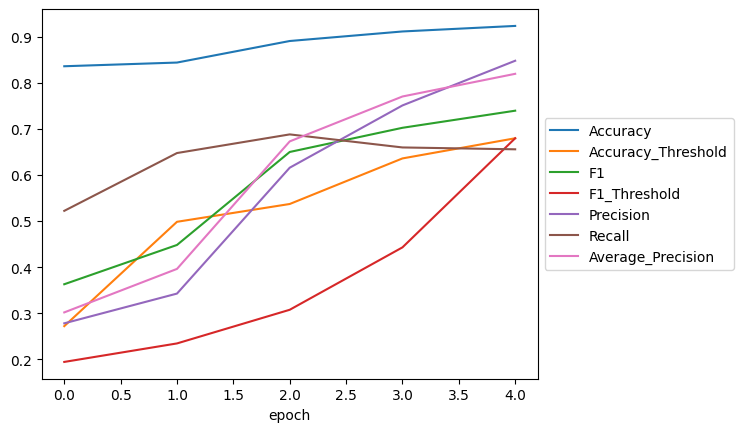
df = pd.read_csv("CEBinaryClassificationEvaluator_results.csv")
df.tail(n=10)
epoch steps Accuracy Accuracy_Threshold F1 F1_Threshold Precision Recall Average_Precision
0 0 -1 0.836230 0.271901 0.362869 0.194206 0.278017 0.522267 0.301740
1 1 -1 0.844251 0.498470 0.448179 0.234365 0.342612 0.647773 0.396195
2 2 -1 0.891043 0.537126 0.650096 0.307447 0.615942 0.688259 0.673045
3 3 -1 0.911765 0.636082 0.702586 0.442940 0.751152 0.659919 0.770558
4 4 -1 0.923797 0.679859 0.739726 0.679859 0.848168 0.655870 0.819789
df.set_index("epoch").drop(columns=["steps"]).plot()
plt.legend(loc='center left', bbox_to_anchor=(1.0, 0.5))
<matplotlib.legend.Legend>

Training considerations

  • Overfitting
  • Architecture
  • Hyperparameter tuning
  • Significance of results

What is a Transformer? (High-level Overview)

Agenda

  1. Transformers 4 IR

  2. Transformer by Examples

  3. Conducting an IR experiment

  4. Analysis - BERTopic Showcase

  5. BERT 4 Reranking - monoBERT (= Cross-encoder)

  6. What is a Transformer? (High-level Overview)

  7. BERT 4 Retrieval - Representation-based (= Bi-encoder)

  8. Discussion

Why transformers:

  • Contextualized embeddings, such as ElMo (2018).
  • Transfer learning, such as ULMFit (2018).
  • Wide-variety of NLP tasks.

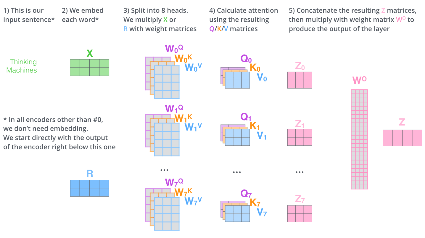
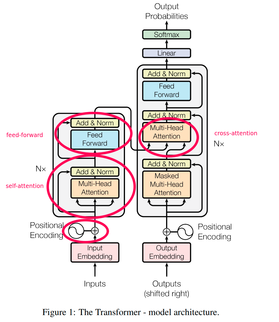
Transformers use multi-head Attention (Attention Is All You Need - 2017):

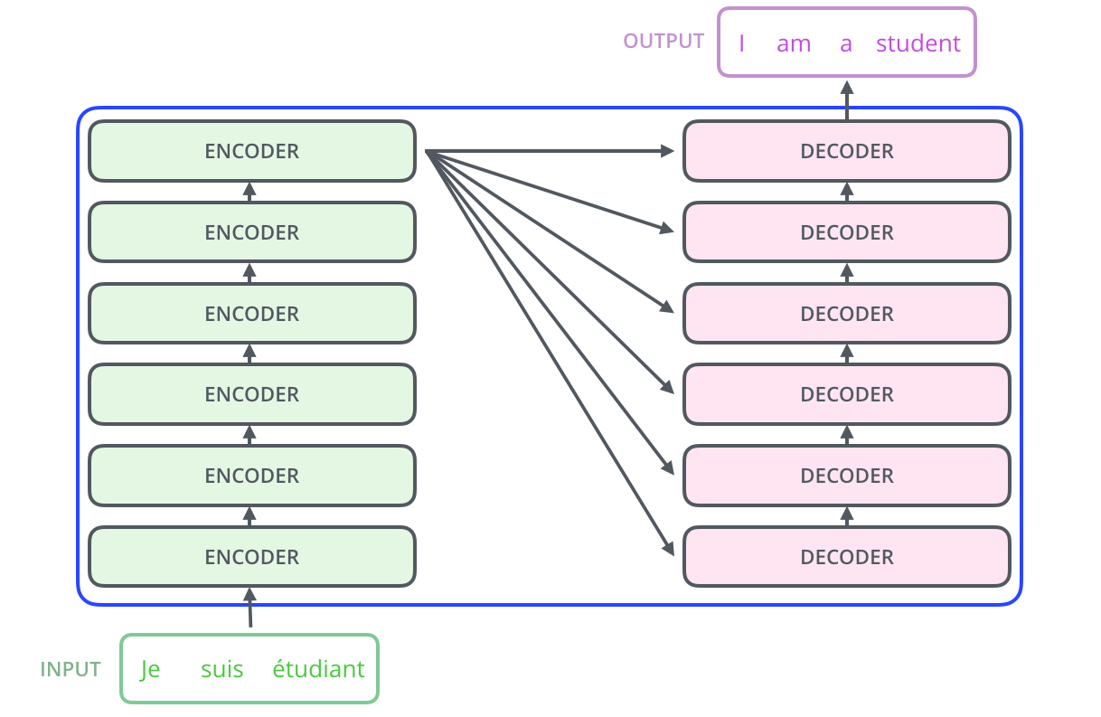
Illustrated Transformer Overview

We end up with an embedding, that can then customized with a special head (e.g., classification or pooling).

Today focus on BERT (2018, bi-directional with masking).

Attention:

\[ softmax(\frac{Q \times K^T}{\sqrt{d_k}})V = Z \]

Note that:

  • Key, Value same source.
  • Query, Key same length.
  • Decoder queries encoder.

from transformers import AutoTokenizer, AutoModel, AutoModelForSequenceClassification

# Tokenizer and model must match
ex_tokenizer = AutoTokenizer.from_pretrained(model_name)
ex_model = AutoModel.from_pretrained(model_name)
ex_model_with_head = AutoModelForSequenceClassification.from_pretrained(model_name)  # Needs fine-tuning, here for demonstration

test_sentences = ["This is the first sentence with complex tokens, such as SentenceTransformers.", "We can batch multiple sentences."]

ex_tokenized = ex_tokenizer(test_sentences, return_tensors="pt", padding=True, truncation=True)  # Collates data with padding
ex_res = ex_model(**ex_tokenized)
ex_res_with_head = ex_model_with_head(**ex_tokenized)
print("\nTokenized text:")  # Word Piece Tokenization
print(ex_tokenizer.tokenize(test_sentences))

Tokenized text:
['this', 'is', 'the', 'first', 'sentence', 'with', 'complex', 'token', '##s', ',', 'such', 'as', 'sentence', '##tra', '##ns', '##form', '##ers', '.', 'we', 'can', 'batch', 'multiple', 'sentences', '.']
print("\nOutput Dictionary:")
print(ex_res.keys())

Output Dictionary:
odict_keys(['last_hidden_state', 'pooler_output'])
print("\nOutput Size:")
print(ex_res.last_hidden_state.size())

Output Size:
torch.Size([2, 20, 384])
print("\nPooled Embeddings (truncated):")
print(ex_res.pooler_output.shape, ex_res.pooler_output[:, :7])

Pooled Embeddings (truncated):
torch.Size([2, 384]) tensor([[-0.0595,  0.0151,  0.0587,  0.0922, -0.0913, -0.0640,  0.0419],
        [ 0.0048,  0.0145,  0.0123,  0.0590, -0.1448, -0.0045, -0.0301]],
       grad_fn=<SliceBackward0>)
print("\nToken IDs:")
print(ex_tokenized)

Token IDs:
{'input_ids': tensor([[  101,  2023,  2003,  1996,  2034,  6251,  2007,  3375, 19204,  2015,
          1010,  2107,  2004,  6251,  6494,  3619, 14192,  2545,  1012,   102],
        [  101,  2057,  2064, 14108,  3674, 11746,  1012,   102,     0,     0,
             0,     0,     0,     0,     0,     0,     0,     0,     0,     0]]), 'token_type_ids': tensor([[0, 0, 0, 0, 0, 0, 0, 0, 0, 0, 0, 0, 0, 0, 0, 0, 0, 0, 0, 0],
        [0, 0, 0, 0, 0, 0, 0, 0, 0, 0, 0, 0, 0, 0, 0, 0, 0, 0, 0, 0]]), 'attention_mask': tensor([[1, 1, 1, 1, 1, 1, 1, 1, 1, 1, 1, 1, 1, 1, 1, 1, 1, 1, 1, 1],
        [1, 1, 1, 1, 1, 1, 1, 1, 0, 0, 0, 0, 0, 0, 0, 0, 0, 0, 0, 0]])}
print("\nContextualized Token Embeddings (truncated):")
print(ex_res.last_hidden_state[:, :3, :7])  # First 3 tokens)

Contextualized Token Embeddings (truncated):
tensor([[[-0.1560, -0.1154,  0.0731,  0.2994,  0.0485,  0.0800,  0.1049],
         [ 0.2525,  0.9195,  0.4429,  0.7421,  0.4402,  0.2827,  1.2313],
         [ 0.0174,  0.3108,  0.0699,  0.3103,  0.2146,  0.4123,  0.3589]],

        [[ 0.1666, -0.2453,  0.0160,  0.0463,  0.0391,  0.0391,  0.2853],
         [ 0.1173, -0.0858,  0.0132, -0.0607,  0.2865,  0.2517,  0.5110],
         [-0.0912, -0.3036, -0.3637,  0.1121,  0.0017,  0.5838,  0.1054]]],
       grad_fn=<SliceBackward0>)
print("\nPredicted Values (not fine-tuning)")
print(ex_res_with_head)

Predicted Values (not fine-tuning)
SequenceClassifierOutput(loss=None, logits=tensor([[0.0310, 0.0070],
        [0.0281, 0.0279]], grad_fn=<AddmmBackward0>), hidden_states=None, attentions=None)

Tokenization

Can be learned. BERT uses WordPiece.
Based on common sub-words (in comparison to word- or character-based).
Can deal with unknown compound words.

Special Tokens

In BERT:
[CLS] sent1 [SEP] sent2 [SEP]

Other tokens:
- [MASK] - [UNK] - [PAD]

# Uses Mean pooling
topic_model.embedding_model.embedding_model
SentenceTransformer(
  (0): Transformer({'max_seq_length': 256, 'do_lower_case': False}) with Transformer model: BertModel 
  (1): Pooling({'word_embedding_dimension': 384, 'pooling_mode_cls_token': False, 'pooling_mode_mean_tokens': True, 'pooling_mode_max_tokens': False, 'pooling_mode_mean_sqrt_len_tokens': False})
  (2): Normalize()
)

Common Pooling Modes

  • Mean Pooling (average)
  • Max Pooling
  • Sequence-length dependant
  • Special token ([CLS] in BERT)
# Starts with embeddings
topic_model.embedding_model.embedding_model[0]._modules["auto_model"]
BertModel(
  (embeddings): BertEmbeddings(
    (word_embeddings): Embedding(30522, 384, padding_idx=0)
    (position_embeddings): Embedding(512, 384)
    (token_type_embeddings): Embedding(2, 384)
    (LayerNorm): LayerNorm((384,), eps=1e-12, elementwise_affine=True)
    (dropout): Dropout(p=0.1, inplace=False)
  )
  (encoder): BertEncoder(
    (layer): ModuleList(
      (0-5): 6 x BertLayer(
        (attention): BertAttention(
          (self): BertSelfAttention(
            (query): Linear(in_features=384, out_features=384, bias=True)
            (key): Linear(in_features=384, out_features=384, bias=True)
            (value): Linear(in_features=384, out_features=384, bias=True)
            (dropout): Dropout(p=0.1, inplace=False)
          )
          (output): BertSelfOutput(
            (dense): Linear(in_features=384, out_features=384, bias=True)
            (LayerNorm): LayerNorm((384,), eps=1e-12, elementwise_affine=True)
            (dropout): Dropout(p=0.1, inplace=False)
          )
        )
        (intermediate): BertIntermediate(
          (dense): Linear(in_features=384, out_features=1536, bias=True)
          (intermediate_act_fn): GELUActivation()
        )
        (output): BertOutput(
          (dense): Linear(in_features=1536, out_features=384, bias=True)
          (LayerNorm): LayerNorm((384,), eps=1e-12, elementwise_affine=True)
          (dropout): Dropout(p=0.1, inplace=False)
        )
      )
    )
  )
  (pooler): BertPooler(
    (dense): Linear(in_features=384, out_features=384, bias=True)
    (activation): Tanh()
  )
)

Types of transformers

BERT only uses Encoder Layers.

  • Encoders (e.g., BERT, RoBERTa): auto-encoding models - NLU
  • Decoders (e.g., GPT): auto-regressive models - NLG
  • Seq2Seq (e.g., BART): encoder-decoder models - Translation

Overview of Models

Transfomer Layers

BERT 4 Retrieval - Representation-based (= Bi-encoder)

Agenda

  1. Transformers 4 IR

  2. Transformer by Examples

  3. Conducting an IR experiment

  4. Analysis - BERTopic Showcase

  5. BERT 4 Reranking - monoBERT (= Cross-encoder)

  6. What is a Transformer? (High-level Overview)

  7. BERT 4 Retrieval - Representation-based (= Bi-encoder)

  8. Discussion

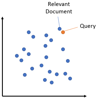
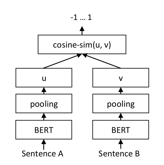
Idea:

  • Train embeddings for queries and documents.
  • Asymmetric architecture vs Siamese network. (we use the latter for simplicity)
  • Similarity function -> loss.
Embedding Based Retrieval Architecture
repBased = SentenceTransformer(model_name)
qs, ds = repBased.encode([{"query": ex0[0]}, {"query": ex1[0]}]), repBased.encode([{"doc": ex0[1]}, {"doc": ex1[0]}])
sentence_transformers.util.cos_sim(qs, ds)
tensor([[0.1819, 0.1325],
        [0.0353, 1.0000]])

Collate Batches

train_ds.set_mode("rep")
valid_ds.set_mode("rep")
train_dl_repBased = DataLoader(train_ds, batch_size=32, collate_fn=repBased.smart_batching_collate)
valid_dl_repBased = DataLoader(valid_ds, batch_size=32, collate_fn=repBased.smart_batching_collate)
assert next(iter(train_dl_repBased))
queries_dict = dict(zip(valid_ds.q_ids, valid_ds.queries))
docs_dict = dict(zip(valid_ds.d_ids, valid_ds.docs))
qrels_dict = valid_ds.qrels

Train

ir_evaluator = sentence_transformers.evaluation.InformationRetrievalEvaluator(queries_dict, docs_dict, qrels_dict, write_csv=True)
repBased.fit(train_objectives=[(train_dl_repBased, losses.CosineSimilarityLoss(repBased))],
          evaluator=ir_evaluator,
          epochs=5, 
          optimizer_class=torch.optim.AdamW,
          show_progress_bar=True,
          save_best_model=True,
          output_path="./",
        )
qs, ds = repBased.encode([{"query": ex0[0]}, {"query": ex1[0]}]), repBased.encode([{"doc": ex0[1]}, {"doc": ex1[0]}])
sentence_transformers.util.cos_sim(qs, ds)
tensor([[0.4993, 0.1709],
        [0.2064, 1.0000]])
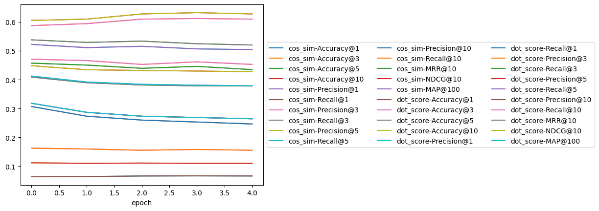
df = pd.read_csv("eval/Information-Retrieval_evaluation_results.csv")
df.tail(n=10)
epoch steps cos_sim-Accuracy@1 cos_sim-Accuracy@3 cos_sim-Accuracy@5 cos_sim-Accuracy@10 cos_sim-Precision@1 cos_sim-Recall@1 cos_sim-Precision@3 cos_sim-Recall@3 ... dot_score-Recall@1 dot_score-Precision@3 dot_score-Recall@3 dot_score-Precision@5 dot_score-Recall@5 dot_score-Precision@10 dot_score-Recall@10 dot_score-MRR@10 dot_score-NDCG@10 dot_score-MAP@100
0 0 -1 0.318386 0.470852 0.538117 0.605381 0.318386 0.307175 0.162930 0.457399 ... 0.307175 0.162930 0.457399 0.112108 0.522422 0.063677 0.587444 0.409075 0.448493 0.412652
1 1 -1 0.286996 0.466368 0.529148 0.609865 0.286996 0.273543 0.159940 0.450673 ... 0.273543 0.159940 0.450673 0.110314 0.511211 0.064574 0.594170 0.389533 0.434542 0.391997
2 2 -1 0.273543 0.452915 0.533632 0.627803 0.273543 0.260090 0.155456 0.439462 ... 0.260090 0.155456 0.439462 0.111211 0.515695 0.066368 0.609865 0.381621 0.432073 0.384038
3 3 -1 0.269058 0.461883 0.524664 0.632287 0.269058 0.253363 0.158445 0.446188 ... 0.253363 0.158445 0.446188 0.110314 0.506726 0.066816 0.612108 0.378787 0.430048 0.381016
4 4 -1 0.264574 0.452915 0.520179 0.627803 0.264574 0.246637 0.155456 0.434978 ... 0.246637 0.155456 0.434978 0.110314 0.504484 0.066368 0.609865 0.378207 0.427841 0.378888

5 rows × 32 columns

df.set_index("epoch").drop(columns=["steps"]).plot(legend=False)
plt.legend(loc='center left', bbox_to_anchor=(1.0, 0.5), ncol=3)
<matplotlib.legend.Legend>

Similarity Search Index

from datasets import Dataset
embs = repBased.encode(list(map(lambda x: {"doc": x}, docs_dict.values())))
dataset = Dataset.from_dict({"id": docs_dict.keys(), "txt": docs_dict.values(), "embeddings": embs})
dataset.add_faiss_index(column='embeddings')
dataset
Dataset({
    features: ['id', 'txt', 'embeddings'],
    num_rows: 1487
})
query = "deep learning transformer models for information retrieval"
q_embeddings = repBased.encode([{"query": query}])[0]
retrieved = dataset.get_nearest_examples('embeddings', query=q_embeddings, k=3)
transformed_scores = 1-retrieved.scores/2  # to cosine similarity, assume normalized
text_snippets = list(map(lambda x: x[:50] + "...", retrieved.examples["txt"]))
retrieved.examples["id"], transformed_scores, text_snippets, np.array(retrieved.examples["embeddings"]).shape
(['859af6e67aec769c58ec1ea6a971108a60df0b9d',
  'a426971fa937bc8d8388e8a657ff891c012a855f',
  '0ad0518637d61e8f4b151657797b067ec74418e4'],
 array([0.7006028 , 0.68879974, 0.68470454], dtype=float32),
 ['Structured Perceptron with Inexact Search: Structu...',
  'Deep Learning for Biomedical Information Retrieval...',
  'Semi-supervised deep learning by metric embedding:...'],
 (3, 384))

Discussion

Agenda

  1. Transformers 4 IR

  2. Transformer by Examples

  3. Conducting an IR experiment

  4. Analysis - BERTopic Showcase

  5. BERT 4 Reranking - monoBERT (= Cross-encoder)

  6. What is a Transformer? (High-level Overview)

  7. BERT 4 Retrieval - Representation-based (= Bi-encoder)

  8. Discussion

Evaluation Considerations

  • Hyperparameter Tuning
  • Final Eval Test Set

Putting things together

  • Multiple re-rankers (e.g., DuoBERT).
  • Evaluate (offline on test data) or online in production system.

Two-Stage Retrieval

Tips and common pitfalls (scaling).

  • CUDA memory errors: start small before scaling up, reduce batch size or text length. More sophisticated methods like gradient accumulation also possible, but require custom training loops.
  • Issues with evaluation (mismatch of questions and experimental setup or data leakage).

Future directions

  • Distillation (Student and Teacher, e.g., distilBERT from HF)
  • Prompt engineering (zero-shot) vs few-shot fine-tuning
  • Contrastive Learning (pretraining or auxiliary tasks) Triplet Loss

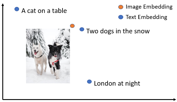
Convergence of Modalities

“A photograph of an astronaut riding a horse” Example Stable Diffusion

Demo freely available: https://huggingface.co/spaces/stabilityai/stable-diffusion

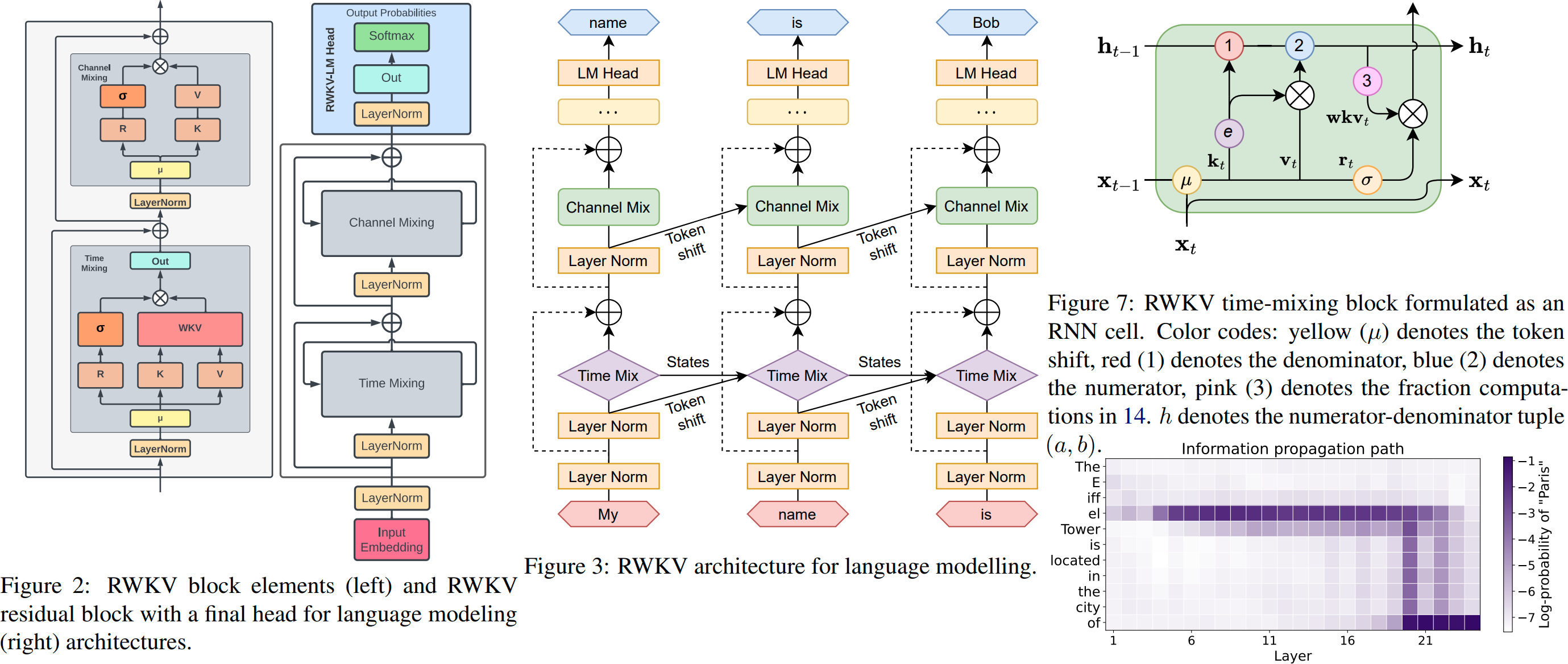
Transformers vs. RNNs

  • Attention vs. State (Time)
  • RWKV

RWKV Picture

Encoder vs. Decoder

  • Training vs. Inference
  • Retrieval-Augmented Generation (RAG)

Vision of LeCun (Godfather, Chief AI Scientist @Meta): JEPA

Further Tasks, Topics

  • Content Bias like framing of messages (e.g., my research focus).
  • Example of solution in shared task of our group - mCPT (1st place in zero-shot Spanish Framing Detection)
  • Question Answering is another common IR-related task tackled with Transformers.
Computational Framing Analysis mCPT

Summary

  • Transformer Conceptually
  • Text Ranking and Retrieval
  • IR Experiment Steps
  • Training and Usage of PyTorch, HuggingFace models, and other libaries
  • Variety of Tasks (Ideas for projects)

Questions?

Next Lectures

Bias and Fairness in Information Retrieval

  • Relates to analysis as seen today

Christmas lecture

  • Invited lecturer